This paper presents a
one-parameter representation of credit risk and transition matrices. We
start with the CreditMetrics view that ratings transition matrices result
from the "binning" of a standard normal random variable
X that
measures changes in creditworthiness. We further assume here that
X
splits into two parts: (1) an idiosyncratic component Y,
unique to a borrower, and (2) a systematic component Z,
shared by all borrowers. Broadly speaking, Z
measures the "credit cycle", meaning the values of default rates and of
end-of-period risk ratings not predicted (using historical average transition
rates) by the initial mix of credit grades. In good years Z
will be positive, implying for each initial credit rating, a lower than
average default rate and a higher than average ratio of upgrades to downgrades.
In bad years, the reverse will be true. We describe a way of estimating
Z
from the separate transition matrices tabulated each year by Standard &
Poor (S&P) and Moody’s. Conversely, we describe a method of calculating
transition matrices conditional on an assumed value for Z.
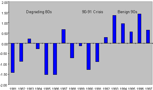
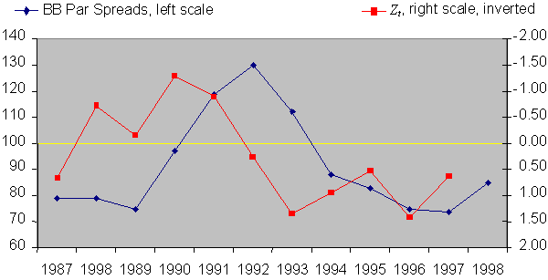
The historical pattern of Z depicts past credit conditions. For example, Z remains negative for most of 1981-89. This mirrors the general decline in credit ratings over that period. In 1990-91, Z drops well below zero as the US suffers through one of its worst credit crises since the Great Depression. The relatively high proportion of lower grade credits inherited from the 1980’s together with the 1990-91 slump (Z<0) accounts for a high number of defaults. Over 1992-97, Z has stayed positive and credit conditions have remained benign. The movements of Z over the past 10 years correlate closely with loan pricing.
Our focus here is on how Zaffects
credit rating migration probabilities. However, one can also model the
effect of Z
on the probability distribution of loss in the event of default (LIED),
credit par spreads, and ultimately the value of a commercial loan, bond,
or other instrument subject to credit risk. By parametrically varying Z,
one can perform stress testing to assess the sensitivity of the value of
an individual credit instrument or an entire credit portfolio to changing
credit conditions. One can also quantify how volatility in Z
translates into transaction and portfolio value volatility.
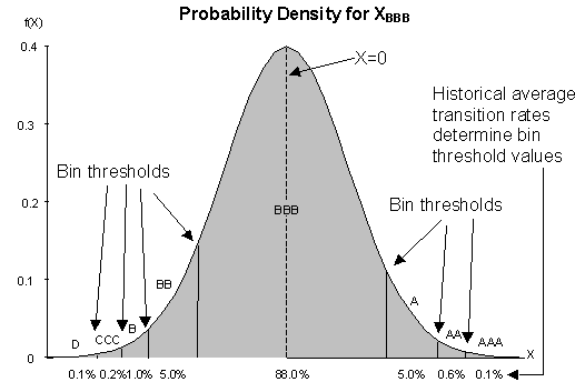
Following the CreditMetrics approach
described by Gupton, Finger, and Bhatia (1997), we assume that ratings
transitions reflect an underlying, continuous credit-change indicator X.
One further assumes that X
has a standard normal distribution. Then, conditional on an initial credit
rating G at the beginning of a year, one partitions X
values into a set of disjoint bins ![]() .
To simplify references, the indices G and g represent sequences of integers
rather than letters or other symbols. One defines the bins so that the
probability that X
falls within a given interval equals the corresponding historical average
transition rate (see Exhibit 1).
.
To simplify references, the indices G and g represent sequences of integers
rather than letters or other symbols. One defines the bins so that the
probability that X
falls within a given interval equals the corresponding historical average
transition rate (see Exhibit 1).
Exhibit 1: Relationship Between Continuous Credit Index X and Rating Transitions

We write the conditions defining the bins as follows:
![]() (1)
(1)
in which P(G,g) denotes the historical average G-to-g transition probability and F (× ) represents the standard normal cumulative distribution function. The default bin has a lower threshold of -¥ . The AAA bin has an upper threshold of +¥ . The remaining thresholds are fit to the observed transition probabilities.
Suppose there are N ratings categories including default. Then there are N-1 initial grades, which represent all the ratings excluding default. For each of those initial grades, we observe N-1 historical average transition rates. (The other (Nth) value derives from the condition that the probabilities sum to 1.) We must determine N-1 threshold values defining the bins. Thus, we can solve for all of the bin boundaries.
We illustrate this process below. The starting point is the smoothed version of the 1981-97 historical average transition matrix tabulated by S&P for 8 grades, including default (see Exhibit 2). The corresponding bins are computed using the above formula.
Consider transitions from BBB. We observe
a 15 bps default rate. Using the inverse probability function for a standard
normal distribution, we compute a value of about –2.97 for the upper threshold
for the default bin. Next consider the CCC bin. We get a value of about
25 bps for the sum of transition rates to CCC or to default. Again
applying the inverse probability function, we get an upper threshold value
for CCC of about –2.81. Now consider B. We compute a probability of about
1.3 per cent for transitions to B or to lower grades. Once again applying
the inverse probability function, we get an upper threshold value of -2.23.
Continuing in this way for each terminal and each initial grade, we derive
all of the bin values.
Exhibit 2: Smoothed Historical Average Transition Rates and Associated Bins
|
|
|
|||||||
|
|
|
|
|
|
|
|
|
|
|
|
||||||||
| AAA |
91.13%
|
8.00%
|
0.70%
|
0.10%
|
0.05%
|
0.01%
|
0.01%
|
0.01%
|
| AA |
0.70%
|
91.03%
|
7.47%
|
0.60%
|
0.10%
|
0.07%
|
0.02%
|
0.01%
|
| A |
0.10%
|
2.34%
|
91.54%
|
5.08%
|
0.61%
|
0.26%
|
0.01%
|
0.05%
|
| BBB |
0.02%
|
0.30%
|
5.65%
|
87.98%
|
4.75%
|
1.05%
|
0.10%
|
0.15%
|
| BB |
0.01%
|
0.11%
|
0.55%
|
7.77%
|
81.77%
|
7.95%
|
0.85%
|
1.00%
|
| B |
0.00%
|
0.05%
|
0.25%
|
0.45%
|
7.00%
|
83.50%
|
3.75%
|
5.00%
|
| CCC |
0.00%
|
0.01%
|
0.10%
|
0.30%
|
2.59%
|
12.00%
|
65.00%
|
20.00%
|
|
|
||||||||
| AAA |
(¥
,-1.35)
|
[-1.35,-2.38)
|
[-2.38,-2.93)
|
[-2.93,-3.19)
|
[-3.19,-3.54)
|
[-3.54,-3.72]
|
[-3.72,-3.89)
|
[-3.89,-¥
)
|
| AA |
(¥
,2.46)
|
[2.46,-1.39)
|
[-1.39,-2.41)
|
[-2.41,-2.88)
|
[-2.88,-3.09)
|
[-3.09,-3.43)
|
[-3.43,-3.72)
|
[-3.72,-¥
)
|
| A |
(¥
,3.10)
|
[3.10,1.97)
|
[1.97,-1.55)
|
[-1.55,-2.35)
|
[-2.35,-2.73)
|
[-2.73,-3.24)
|
[-3.24,-3.29)
|
[-3.29,-¥
)
|
| BBB |
(¥
,3.50)
|
[3.50,2.73)
|
[2.73,1.56)
|
[1.56,-1.55)
|
[-1.55,-2.23)
|
[-2.23,-2.81)
|
[-2.81,-2.97)
|
[-2.97,-¥
)
|
| BB |
(¥
,3.89)
|
[3.89,3.05)
|
[3.05,2.48)
|
[2.48,1.38)
|
[1.38,-1.29)
|
[-1.29,-2.09)
|
[-2.09,-2.33)
|
[-2.33,-¥
)
|
| B |
(¥
,4.11)
|
[4.11,3.29)
|
[3.29,2.75)
|
[2.75,2.43)
|
[2.43,1.42)
|
[1.42,-1.36)
|
[-1.36,-1.64)
|
[-1.64,-¥
)
|
| CCC |
(¥
,4.27)
|
[4.27,3.72)
|
[3.72,3.06)
|
[3.06,2.64)
|
[2.64,1.88)
|
[1.88,1.04)
|
[1.04,-0.84)
|
[-0.84,-¥
)
|
As in Belkin, Suchower, and Forest (1998), we decompose X into two parts: (1) a (scaled) idiosyncratic component Y, unique to a borrower, and (2) a (scaled) systematic component Z, shared by all borrowers. Thus, we write
![]() (2)
(2)
We assume that Y and Z are unit normal random variables and mutually independent. The parameter r (assumed positive) represents the correlation between Z and X. Thus Z explains a fraction r of the variance of X.
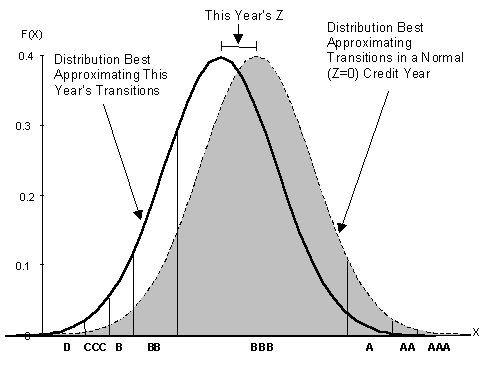
In any year, the observed transition rates will deviate from the norm (Z =0). We can then find a value of Z so that the probabilities associated with the bins defined above best approximate the given year’s observed transition rates (see Exhibit 3). We label that value of Z for year t, Zt. We determine Ztso as to minimize the weighted, mean-squared discrepancies between the model transition probabilities and the observed transition probabilities.
For this we define
 (3)
(3)
This is the model value for the G-to-g
transition rate in year t. Then for a fixed ![]() and a fixed t, the least-squares problem takes the form
and a fixed t, the least-squares problem takes the form
 (4)
(4)
where Pt(G,g) represents the G-to-g transition rate observed in year t and nt,G is the number of transitions from initial grade G observed in that year. In this formula, we weight observations by the inverses of the approximate sample variances of Pt(G,g).
Exhibit 3: Illustration of the Z Value for a Particular Initial Rating in a Given Year

We don’t know the value of r a priori. We estimate r as follows. We apply the minimization in (4) for 1981-97 using an assumed value of r . We then obtain a time series for Zt, conditional on r . We compute the mean and variance of this series. We repeat this process for many values of r , and use a numerical search procedure to find the particular r value for which the Zt time series has variance of one.
We illustrate this process of solving for Zt at a single time t. We start with the S&P transition matrix observed for 1982 (see Exhibit 4). We hold fixed the bins determined from the historical average matrix and fix r at the value (.0163) determining by the search process. The indicated value for Zt of –0.89 provides the best fit to the observed 1982 transition rates.
Exhibit 4: S&P Transition Matrix for 1982 and Calculations Leading to Z Estimate
|
|
|
|
|||||||
|
|
|
|
|
|
|
|
|
|
|
|
|
|||||||||
| AAA |
85
|
92.94%
|
4.71%
|
2.35%
|
0.00%
|
0.00%
|
0.00%
|
0.00%
|
0.00%
|
| AA |
220
|
0.46%
|
92.52%
|
6.08%
|
0.47%
|
0.47%
|
0.00%
|
0.00%
|
0.00%
|
| A |
480
|
0.00%
|
4.45%
|
84.95%
|
9.54%
|
0.64%
|
0.00%
|
0.00%
|
0.42%
|
| BBB |
298
|
0.37%
|
0.37%
|
3.26%
|
85.52%
|
9.78%
|
0.37%
|
0.00%
|
0.34%
|
| BB |
168
|
0.00%
|
0.68%
|
0.00%
|
2.68%
|
82.42%
|
10.05%
|
0.00%
|
4.17%
|
| B |
161
|
0.00%
|
0.00%
|
0.72%
|
0.72%
|
2.89%
|
87.50%
|
5.06%
|
3.11%
|
| CCC |
16
|
0.00%
|
0.00%
|
0.00%
|
0.00%
|
0.00%
|
7.39%
|
73.86%
|
18.75%
|
|
|
|||||||||
| AAA |
85
|
89.34%
|
9.54%
|
0.89%
|
0.13%
|
0.07%
|
0.01%
|
0.01%
|
0.01%
|
| AA |
220
|
0.48%
|
89.56%
|
8.93%
|
0.77%
|
0.13%
|
0.09%
|
0.03%
|
0.01%
|
| A |
480
|
0.06%
|
1.72%
|
90.88%
|
6.14%
|
0.78%
|
0.34%
|
0.01%
|
0.07%
|
| BBB |
298
|
0.01%
|
0.20%
|
4.39%
|
88.03%
|
5.72%
|
1.33%
|
0.13%
|
0.20%
|
| BB |
168
|
0.00%
|
0.07%
|
0.38%
|
6.19%
|
81.63%
|
9.39%
|
1.06%
|
1.29%
|
| B |
161
|
0.00%
|
0.03%
|
0.17%
|
0.32%
|
5.56%
|
83.41%
|
4.38%
|
6.14%
|
| CCC |
16
|
0.00%
|
0.01%
|
0.06%
|
0.20%
|
1.94%
|
10.09%
|
64.53%
|
23.16%
|
| Z Value |
|
||||||||
Broadly speaking, Zt
measures the "credit cycle," meaning the values of default rates and of
end-of-period risk ratings not predicted (using historical average transition
rates) by the initial mix of credit grades. In good years Zt
will be positive, implying for each initial credit rating a lower than
average default rate and a higher than average ratio of upgrades to downgrades.
In bad years, the reverse will be true.
Zt’s historical movements describe past credit conditions not evident in the initial mix of ratings (see Exhibit 5). Zt’s history is erratic, more so than the term "credit cycle" suggests. In particular, the fluctuations don’t show a stable sinusoidal pattern.
Exhibit 5: Zt as Estimated from S&P Annual Transition Matrices

Zt is mostly negative over 1981-89. Credit ratings generally declined over that period as many corporations increased leverage. In 1990-91, Zt drops below zero, as the US suffers through one of its worst credit crises since the Great Depression. The relatively high proportion of lower grade credits inherited from the 1980’s together with the 1990-91 credit slump (Zt<0) accounts for a high number of defaults. Over the period 1992-97, Zt has stayed positive and credit conditions have remained benign.
Loan prices over the past 10 years
correlate quite closely with the credit indicator Zt
(see Exhibit 6). One observes that loan spreads have generally lagged abrupt
changes in credit conditions.
Exhibit 6: Zt Index and BB Spreads

Loan spreads in North America and Europe over the past 2-3 years have remained near record lows. This suggests that the past 6 years of favorable credit conditions have made many lenders optimistic about the future. One might ask whether the past patterns exhibited by Zt justify this optimism or any other forecast of credit conditions.
Applying the weighted least-squares scheme for estimating the Zt, we get a r value of 0.0163. Thus, systematic credit migration risk accounts for only about 1.6% of total credit migration risk over the period 1981-97. This contrasts with equity price data, which suggest that systematic risk accounts for about 25 per cent of the total variance in an average company’s stock price. We shall see below, however, that small variations in Zt can translate into substantial swings in default and downgrade rates.
The discrete time counterpart to the O-U model is a first-order autoregressive process. We fitted such a model for Zt to the data for the 1982-97 period and obtained the following:
![]() (5)
(5)
Here ![]() is a standardized white noise sequence. From (5), the sample estimates
for the O-U model parameters are
is a standardized white noise sequence. From (5), the sample estimates
for the O-U model parameters are ![]() and
and ![]() . Thus,
the Zt
process has an estimated mean relaxation time of about 2 years and an estimated
annual volatility of about 100%.
. Thus,
the Zt
process has an estimated mean relaxation time of about 2 years and an estimated
annual volatility of about 100%.
We performed several statistical tests
on (5) for model goodness of fit. The sample estimate of the mean of the
Zt
process
mean is ![]() ,
with a standard error of 0.25. As a result, there is no statistical basis
to reject the hypothesis that the Zt
process has zero mean. Based on a t-statistic value of 2.18, the hypothesis
that there is no mean reversion (i.e., that
,
with a standard error of 0.25. As a result, there is no statistical basis
to reject the hypothesis that the Zt
process has zero mean. Based on a t-statistic value of 2.18, the hypothesis
that there is no mean reversion (i.e., that ![]() )
can be rejected at the .025 significance level. The Kolmogorov-Smirnov
test statistic for the model residuals has a value of
)
can be rejected at the .025 significance level. The Kolmogorov-Smirnov
test statistic for the model residuals has a value of ![]() ,
indicating that the residuals are statistically indistinguishable from
a white noise sequence
,
indicating that the residuals are statistically indistinguishable from
a white noise sequence ![]() .
.
The calculated R2 for the
model in (5) is .24, indicating that a first-order autoregressive model
for the Zt has
modest predictive power. However, the utility of the model is not in predicting
future values of Zt.
Rather, it is to quantify how the variability in Zt
that is predictable and the variability in Zt
that is not predictable each influence credit risk and the pricing of that
risk.
We again use the bin values ![]() for each initial grade G and end-of-year grade g. Now, conditional on Zt,
we compute the probability of a G to g transition as
for each initial grade G and end-of-year grade g. Now, conditional on Zt,
we compute the probability of a G to g transition as
 (6)
(6)
We show matrices below for a good year
(Zt
=1), an average year (Zt
=0), and a bad year (Zt
=-1) (see Exhibit 7). Note that an absolute value of 1 represents a 1-standard
deviation variation from "normal" credit conditions.
Exhibit 7: Transition Matrices Computed Using Z Parameterization
|
|
|
|||||||
|
|
|
|
|
|
|
|
|
|
|
|
||||||||
| AAA |
93.17%
|
6.25%
|
0.47%
|
0.06%
|
0.03%
|
0.01%
|
0.00%
|
0.00%
|
| AA |
0.95%
|
92.72%
|
5.81%
|
0.41%
|
0.06%
|
0.04%
|
0.01%
|
0.01%
|
| A |
0.14%
|
3.02%
|
92.33%
|
3.88%
|
0.42%
|
0.17%
|
0.01%
|
0.03%
|
| BBB |
0.03%
|
0.41%
|
7.03%
|
88.00%
|
3.65%
|
0.73%
|
0.06%
|
0.09%
|
| BB |
0.01%
|
0.15%
|
0.73%
|
9.50%
|
82.00%
|
6.32%
|
0.61%
|
0.67%
|
| B |
0.00%
|
0.07%
|
0.34%
|
0.59%
|
8.58%
|
83.68%
|
3.03%
|
3.70%
|
| CCC |
0.00%
|
0.01%
|
0.14%
|
0.40%
|
3.30%
|
14.12%
|
65.60%
|
16.42%
|
|
|
||||||||
| AAA |
91.31%
|
7.87%
|
0.67%
|
0.09%
|
0.05%
|
0.01%
|
0.00%
|
0.00%
|
| AA |
0.66%
|
91.24%
|
7.34%
|
0.57%
|
0.09%
|
0.06%
|
0.02%
|
0.01%
|
| A |
0.09%
|
2.26%
|
91.79%
|
4.98%
|
0.58%
|
0.24%
|
0.01%
|
0.05%
|
| BBB |
0.02%
|
0.28%
|
5.52%
|
88.28%
|
4.66%
|
1.01%
|
0.09%
|
0.14%
|
| BB |
0.00%
|
0.10%
|
0.52%
|
7.63%
|
82.13%
|
7.84%
|
0.82%
|
0.95%
|
| B |
0.00%
|
0.04%
|
0.23%
|
0.43%
|
6.87%
|
83.85%
|
3.71%
|
4.86%
|
| CCC |
0.00%
|
0.01%
|
0.09%
|
0.28%
|
2.51%
|
11.91%
|
65.39%
|
19.81%
|
|
|
||||||||
| AAA |
89.09%
|
9.75%
|
0.92%
|
0.14%
|
0.07%
|
0.01%
|
0.01%
|
0.01%
|
| AA |
0.46%
|
89.34%
|
9.13%
|
0.79%
|
0.14%
|
0.10%
|
0.03%
|
0.01%
|
| A |
0.06%
|
1.66%
|
90.75%
|
6.28%
|
0.80%
|
0.35%
|
0.01%
|
0.07%
|
| BBB |
0.01%
|
0.19%
|
4.27%
|
87.96%
|
5.85%
|
1.37%
|
0.14%
|
0.21%
|
| BB |
0.00%
|
0.07%
|
0.37%
|
6.03%
|
81.53%
|
9.58%
|
1.09%
|
1.33%
|
| B |
0.00%
|
0.03%
|
0.16%
|
0.31%
|
5.42%
|
83.32%
|
4.47%
|
6.30%
|
| CCC |
0.00%
|
0.00%
|
0.06%
|
0.20%
|
1.88%
|
9.88%
|
64.39%
|
23.58%
|
One observes significant variation in the migration probabilities between the good, average, and bad years, particularly off the main diagonal. For example, the default probability starting in grade B is .050 in an average year but increases to .068 in a bad year and drops to .036 in a good year. In relative terms these are about 30% variations. Consequently, the effect of systematic risk on migration probabilities is significant.
5. Applications
The Z variable and its related formulas provide a simple one-factor description of credit portfolio risk and credit pricing. On the pricing side, changes in credit spreads for a given grade reflect shifting expectations regarding expected and unexpected loss. By "unexpected loss," we mean the premium (over expected loss) that a loan must pay to compensate for its contribution to volatility in a well-diversified portfolio.
We can explain changes in credit spreads using Z. Suppose that the expected value of Z increases. Then the anticipated transition rates to default and to near default go down. The probability distribution for LIED can shift downward (and change shape) as well. The effect is that both expected and unexpected losses fall, lowering credit spreads. Suppose, alternatively, that the expected value of Z decreases. Expected and unexpected losses go up, raising credit spreads. Thus, we can relate spread volatility to changes in expected credit conditions.
Given a stochastic specification for Z, we can incorporate spread volatility into loan pricing models. We’re currently modifying KPMG’s Loan Analysis SystemSM by incorporating Z risk along with its effect on rating migration probabilities, on the distribution of LIED, and on par credit spreads. In addition, we are including Z risk as one of the factors in a multifactor model for the interest rate term structure.
The Z variable provides a simple way of running credit scenarios. For example, one might want to simulate the value of a credit portfolio under conditions similar to those in 1990-91. To accomplish this, one would run a two-year simulation, setting Z equal to its 1990 value in year 1 and to its 1991 value in year 2. One would compute the associated transition matrices and use those matrices in calculating credit value-at-risk.
Alternatively, one could run a large number of simulations drawing Z from a time series model, such as the O-U process. This would provide valuable insight into how volatility in Z in response to changing credit conditions induces volatility in the mark-to-market value of a credit portfolio.
In closing, note that Z offers only a one-factor explanation of credit risk. International data suggest that one needs several factors to describe credit risk globally. The assumption that a single factor can satisfactorily represent all systematic risk in valuing a credit portfolio needs to be tested by comparing model predictions of mark-to-market prices with observed market prices.
6. Summary
We have described a one-parameter representation of credit risk and transition matrices in the form of a single systematic credit factor Z. The historical record of Z provides a succinct description of past credit conditions. We have described a stochastic process model for Z and a way of estimating Z from past ratings transition matrices and applied the method to rating migration data for the period 1983-97.
Our results indicate that specific risk dominates systematic risk in terms of explaining the variance of X, the continuous variate that governs credit migration under the CreditMetrics model. Nonetheless, Z has a significant effect on migration probabilities, and the framework that we described can be used to stress test a credit portfolio, i.e., to quantify the impact of changing credit conditions on individual transaction value and portfolio value.
The Z variate can be incorporated into models for stochastic LIED and stochastic par credit spreads. It also provides a basis for modeling the correlation between credit migration and interest rates, foreign currency exchange rates, and other market variables subject to systematic risk.
References
Arnold, Ludwig. Stochastic Differential Equations: Theory and Applications. John Wiley & Sons, 1974.
Belkin, Barry, Stephan J. Suchower, and Lawrence R. Forest, Jr. J.P. Morgan CreditMetrics®.Monitor. First Quarter 1998.
Gupton, Greg, M., Christopher C. Finger, and Mickey Bhatia. CreditMetricsTM – Technical Document. New York: Morgan Guaranty Trust Co., 1997.