Value at Risk and on Loan Pricing
Barry Belkin, Daniel H. Wagner Associates
Larry Forest, KPMG Peat Marwick
The CreditMetricsTM methodology
incorporates a model for the correlation between the rating grade migrations
of different borrowers. In the context of commercial lending, we investigate
the effects of the systematic credit risk which this migration correlation
induces. In Section I we consider the impact systematic credit risk has
on loan portfolio value at risk. In Section II our focus shifts to individual
loan transactions and the effect of systematic risk on credit spreads.
Our results demonstrate the importance of properly accounting for systematic
risk at both the loan portfolio level and loan transaction level.
I. Systematic Credit Risk at the Loan Portfolio Level
In modeling credit migration correlation, we follow the CreditMetricsTM approach described in [1] and assume that rating transitions in discrete grade are induced by migration in an underlying process which measures "distance" from default. We assume the appropriate nonlinear transformation is made between this default distance and a normalized risk score so that one-period changes in normalized score have a unit normal distribution.
We index borrowers by i and
let ![]() denote
the one-period normalized risk score change of borrower
denote
the one-period normalized risk score change of borrower ![]() .
To account for migration correlation, we assume that each
.
To account for migration correlation, we assume that each ![]() has a one-factor decomposition of the form:
has a one-factor decomposition of the form:
The essential property of ![]() -risk
is that it is diversifiable and therefore commands no risk premium. On
the other hand, Z-risk is common to every portfolio of loans, no matter
how large and well balanced. Because it can not be diversified away, it
is Z-risk which accounts for the credit risk premium that lenders charge
for "unexpected" credit loss.
-risk
is that it is diversifiable and therefore commands no risk premium. On
the other hand, Z-risk is common to every portfolio of loans, no matter
how large and well balanced. Because it can not be diversified away, it
is Z-risk which accounts for the credit risk premium that lenders charge
for "unexpected" credit loss.
The relative weighting of Z-risk
and ![]() -risk in the decomposition
of the
-risk in the decomposition
of the ![]() is defined so that
is defined so that ![]() is the correlation between
is the correlation between ![]() and
and ![]() for
for ![]() .
We restrict the correlation between borrowers to be non-negative, so that
.
We restrict the correlation between borrowers to be non-negative, so that ![]() .
The extreme cases are: (i)
.
The extreme cases are: (i) ![]() -risk
only (
-risk
only (![]() ) with
all credit risk diversifiable and (ii) Z-risk only (
) with
all credit risk diversifiable and (ii) Z-risk only (![]() )
with all risk systematic.
)
with all risk systematic.
The boundaries between adjacent
rating grades are determined by breakpoints ![]() .
The defining property of the
.
The defining property of the ![]() is that the probabilities for one-period transitions between letter grades
which result from Equation (1) should agree with observed transition probabilities.
We note that this method of calibrating the factor model in Equation (1)
results in a distinctly different set of rating grade breakpoints for each
starting grade.
is that the probabilities for one-period transitions between letter grades
which result from Equation (1) should agree with observed transition probabilities.
We note that this method of calibrating the factor model in Equation (1)
results in a distinctly different set of rating grade breakpoints for each
starting grade.
Consider a two-period simple (option-free)
term loan L and let X denote the payoff to the lender at the end of the
first period. We apply the standard variance decomposition formula to X:
![]() .
(2)
.
(2)
Here the term ![]() is the average level of payoff variability induced by
is the average level of payoff variability induced by ![]() and is therefore a measure of (diversifiable)
and is therefore a measure of (diversifiable) ![]() -risk.
The term
-risk.
The term ![]() ,
on the other hand, is a measure of the systematic variability in loan payoff
induced by Z-risk.
,
on the other hand, is a measure of the systematic variability in loan payoff
induced by Z-risk.
Consider now a loan portfolio ![]() comprised of a large number N of loans contractually identical to L but
made to different borrowers, each with the same initial rating grade. Let
SN denote the portfolio payoff of
comprised of a large number N of loans contractually identical to L but
made to different borrowers, each with the same initial rating grade. Let
SN denote the portfolio payoff of ![]() .
Since the payoffs of the loans in
.
Since the payoffs of the loans in ![]() are conditionally independent given Z, it follows that
are conditionally independent given Z, it follows that
![]() (3)
(3)
Observe that the systematic risk
term in the variance decomposition of ![]() scales with
scales with ![]() ,
while the diversifiable risk term scales with
,
while the diversifiable risk term scales with ![]() .
The implication is that as long as there is some positive correlation between
borrowers in their rating migrations, then for large enough
.
The implication is that as long as there is some positive correlation between
borrowers in their rating migrations, then for large enough ![]() the systematic risk will dominate in the variance decomposition
the systematic risk will dominate in the variance decomposition
To address this question, we implemented
a spreadsheet which calculates the probability distribution for the payoff
of a portfolio of two-period loans. Specifically, we set ![]() and determined the distribution for the normalized portfolio net present
value. The NPV normalization consists of a change of location to center
at
and determined the distribution for the normalized portfolio net present
value. The NPV normalization consists of a change of location to center
at ![]() and
a change of scale which divides by
and
a change of scale which divides by ![]() .
The resulting variate represents the unexpected portfolio gain or loss
measured in units of standard deviation. It is through this normalized
variate that we quantify portfolio value at risk.
.
The resulting variate represents the unexpected portfolio gain or loss
measured in units of standard deviation. It is through this normalized
variate that we quantify portfolio value at risk.
The assumed loan parameters and model inputs for the two-year loan are:
• One-year rating grade transition matrix taken from Moody’s Report (see [4])
• Constant risk-free interest rate = 4.5%
• No loan origination or holding cost
• Loss in the event of default = ![]()
• Credit risk premiums with a flat term structure:
Aaa: 3.0 bps, Aa: 4.8 bps, A: 10.0 bps, Baa: 16.0 bps, Ba: 120.0 bps, B: 150.0 bps, Caa: 300.0 bps
• Credit migration correlation ![]() .
.
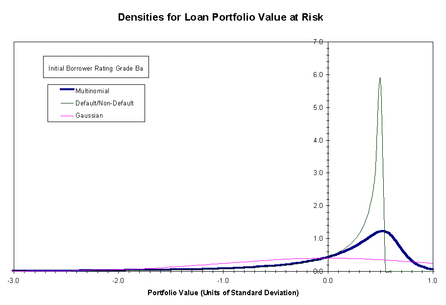
For purposes of comparison, we have
also displayed the density ![]() that one obtains by assigning the two-period loan the value $1 (par value)
at the end of period 1 if the loan does not default during period 1 and
the value
that one obtains by assigning the two-period loan the value $1 (par value)
at the end of period 1 if the loan does not default during period 1 and
the value ![]() if the loan
defaults. This method of valuation accounts for systematic risk but effectively
collapses the full-state migration process to two rating states: default
and non-default. The mean portfolio payoff under the default/non-default
model turns out to be $10,116.25, a very close approximation to the $10,116.10
obtained under the full-state model. However, the portfolio payoff standard
deviation under the default/non-default model is $83.26, a significant
underestimate of the actual standard deviation of $96.00.
if the loan
defaults. This method of valuation accounts for systematic risk but effectively
collapses the full-state migration process to two rating states: default
and non-default. The mean portfolio payoff under the default/non-default
model turns out to be $10,116.25, a very close approximation to the $10,116.10
obtained under the full-state model. However, the portfolio payoff standard
deviation under the default/non-default model is $83.26, a significant
underestimate of the actual standard deviation of $96.00.
The density ![]() is the unit Gaussian density that one would obtain for normalized value
at risk if the rating migration processes of the borrowers were statistically
independent. In that case, the central limit theorem would apply uncon-ditionally
and the density for the normalized portfolio payoff would be closely approximated
as unit normal.
is the unit Gaussian density that one would obtain for normalized value
at risk if the rating migration processes of the borrowers were statistically
independent. In that case, the central limit theorem would apply uncon-ditionally
and the density for the normalized portfolio payoff would be closely approximated
as unit normal.
Both ![]() and
and ![]() are
observed to be markedly asymmetric with respect to their mean values and
to have modes that are skewed to the right. The mode of
are
observed to be markedly asymmetric with respect to their mean values and
to have modes that are skewed to the right. The mode of ![]() is more narrowly peaked than that of
is more narrowly peaked than that of ![]() .
The upper tail of
.
The upper tail of ![]() is sharply truncated. There are also differences in the lower tails of
the two densities that are not discernible at the scale shown. Consider,
for example, the probability of a portfolio loss. The expected portfolio
profit of $116.10 is equal to
is sharply truncated. There are also differences in the lower tails of
the two densities that are not discernible at the scale shown. Consider,
for example, the probability of a portfolio loss. The expected portfolio
profit of $116.10 is equal to ![]() .
Under
.
Under ![]() the
probability of a payoff outcome that falls
the
probability of a payoff outcome that falls ![]() or more below the mean is .080. The corresponding probability of a portfolio
loss under
or more below the mean is .080. The corresponding probability of a portfolio
loss under ![]() is .065. So the use of
is .065. So the use of ![]() as a proxy for
as a proxy for ![]() would result in an underestimate of the probability of a portfolio loss.
would result in an underestimate of the probability of a portfolio loss.
As one would expect, the comparison
between ![]() and the unit normal density (which completely ignores the effect of systematic
risk) is even more striking. The density
and the unit normal density (which completely ignores the effect of systematic
risk) is even more striking. The density ![]() has none of the symmetry of the Gaussian density and, as in the comparison
with
has none of the symmetry of the Gaussian density and, as in the comparison
with ![]() , has
a heavier lower tail. If the portfolio payoff density were well-approximated
as Gaussian, then the probability of a portfolio loss would be .113. This
is now an overestimate for the actual loss probability of .080.
, has
a heavier lower tail. If the portfolio payoff density were well-approximated
as Gaussian, then the probability of a portfolio loss would be .113. This
is now an overestimate for the actual loss probability of .080.
Our results show then that failure to discriminate among non-default grades in modeling rating migration and failure to account for systematic credit risk can both lead to significant errors in the portfolio value-at-risk density.
Figure 1
II. Systematic Credit Risk at the Loan Transaction Level
The issue of how to treat systematic credit risk at the loan transaction level arises in the application of arbitrage methods to loan pricing. The point is made in [3] in the finite (discrete time and discrete risk rating) model context that only "binomial" credit risks can be uniquely priced by arbitrage. These are risks where default and non-default are the only distinguished credit states. The issue then becomes how to price the "multinomial" risks that arise when the non-default state is split into multiple risk grades.
The approach taken in [3] is to introduce one-period binomial reference loans whose payoffs statistically approximate the one-period payoffs of the actual loan. The specific calibration is to choose the reference loan payoffs so that the the mean and variance of the payoff distribution exactly match the corresponding moments of the one-period payoff distribution of the actual loan. For reasons that will be made clear below, we refer to this calibration scheme as the total risk method. Each reference loan, having only two possible payoff values, can be priced uniquely by arbitrage. A recursive procedure is then used to price the actual loan in terms of the reference loans.
A comparison is made in [3] between
an hypothesized portfolio ![]() of N statistically identical loans, each with the actual multinomial
payoff distribution, and a counterpart portfolio
of N statistically identical loans, each with the actual multinomial
payoff distribution, and a counterpart portfolio ![]() of N statistically identical loans whose payoffs are those of the
associated reference loans. It is then argued that the value of portfolio
of N statistically identical loans whose payoffs are those of the
associated reference loans. It is then argued that the value of portfolio ![]() and the value of portfolio
and the value of portfolio ![]() must approach asymptotic equality as
must approach asymptotic equality as ![]() .
The key to the argument is the application of the central limit theorem.
.
The key to the argument is the application of the central limit theorem.
However, the assumption of statistical independence in this context is problematic. If arbitrarily large portfolios of independent but statistically identical loans could actually be constructed, the credit risks being priced would be fully diversifiable and would command no market premium. This is inconsistent with the fact that the loan spreads observed in the market incorporate a component for unexpected credit loss as well as a component for expected credit loss. The market must therefore be acting as though there is systematic credit risk underlying the rating grade migration processes of different borrowers.
The question then becomes how to properly modify the reference loan calibration to account for systematic credit risk. The variance decomposition in Equation (2) above provides the answer. We have observed that it is systematic risk that commands a risk premium. Therefore, if two credit risks are to be priced the same by the market, they should have the same amount of systematic risk. The calibration in [3] should therefore be based on matching the systematic component of variance of the reference loan payoffs to the systematic component of variance of the actual loan payoffs. We refer to this scheme as the systematic risk method.
We have implemented a spreadsheet which applies both the total risk method and the alternative systematic risk method to a two-period term loan. The value of the systematic risk variate Z is discretized into 1,000 equiprobability bins. The required conditional moments are determined both for the payoff distribution of an individual loan and the payoff distribution of a portfolio of 10,000 loans statistically identical to the given loan. Strong use is made in the calculations of the conditional independence of the portfolio loan payoffs for each value of Z.
We applied the total variance decomposition
to the previously described two-period loan with the borrower initially
in rating grade Ba and a (par) credit spread of 171.9 bps and with ![]() .
The results are shown in the following two tables.
.
The results are shown in the following two tables.
The values in Table 1 indicate that
at the individual loan level most of the payoff variance (about 95%) is
attributable to diversifiable risk. If the total risk calibration scheme
is used, the systematic variance of the binomial reference loan payoff
distribution underestimates the systematic variance of the actual loan
payoff distribution. We observed this to be the case for all initial rating
grades and for varying values of the correlation parameter ![]() .
.
At the portfolio level, Table 2 shows that virtually all of the payoff variance (99.7%) is attributable to systematic risk. Furthermore, at the portfolio level there is now a significant mismatch in total variance. Consequently, the second-order match between the binomial loan payoffs and the actual loan payoffs that was enforced at the transaction level is not preserved at the portfolio level.
Table 1
Variance Decomposition: Individual Loan
|
|
|
|
| $1.011610 | $1.011610 | |
| .001750 | .001772 | |
| .000092 | .000069 | |
| .001842 | .001841 | |
| $.042913 | $.042912 |
Table 2
Variance Decomposition: Loan Portfolio
|
|
|
|
| $10,116.10 | $10,116.10 | |
| 17.50 | 17.72
|
|
| 9,197.68 | 6,913.57
|
|
| 9,215.18 | 6,931.29 | |
| $96.00
|
$83.25
|
To provide further insight, in the
four figures which follow, we show the (normalized) portfolio payoff densities
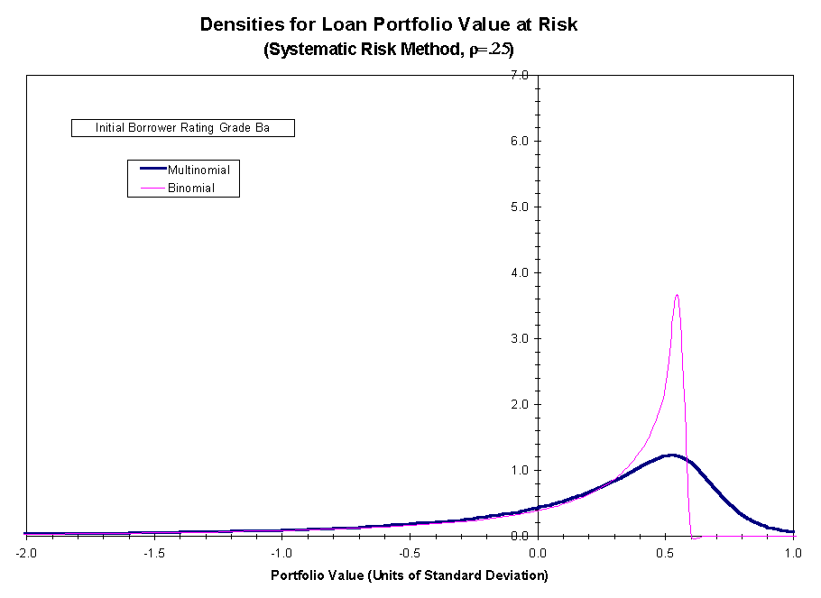
for initial risk grade Ba and two levels of the credit migration
correlation, ![]() and
and ![]() . Figures
2 and 3 apply to the case
. Figures
2 and 3 apply to the case ![]() .
In Figure 2, we compare the normalized portfolio value-at-risk density
for the actual loan payoff with the corresponding reference loan payoff
density calculated based on the total risk method of calibration. Figure
3 shows the analogous comparison, but with the reference loan payoff density
calculated using the systematic risk method of calibration. Figures 4 and
5 show the analogous comparison between the two methods of risk calibration
for
.
In Figure 2, we compare the normalized portfolio value-at-risk density
for the actual loan payoff with the corresponding reference loan payoff
density calculated based on the total risk method of calibration. Figure
3 shows the analogous comparison, but with the reference loan payoff density
calculated using the systematic risk method of calibration. Figures 4 and
5 show the analogous comparison between the two methods of risk calibration
for ![]() .
.
The principle involved here is that
the closer the portfolios ![]() and
and ![]() are in their payoff
distributions, the closer the common price of the loans in
are in their payoff
distributions, the closer the common price of the loans in ![]() must be to the common price of the loans in
must be to the common price of the loans in ![]() .
The figures show that the agreement between the payoff distributions for
the portfolios
.
The figures show that the agreement between the payoff distributions for
the portfolios ![]() and
and ![]() is closer (but still not exact) if the calibration is based on systematic
risk as opposed to total risk.
is closer (but still not exact) if the calibration is based on systematic
risk as opposed to total risk.
This improvement is observed both
when ![]() and
when
and
when ![]() .
In each case, the locations of the density peaks become better aligned
and the disparity in peak height diminishes, more significantly one observes,
when
.
In each case, the locations of the density peaks become better aligned
and the disparity in peak height diminishes, more significantly one observes,
when ![]() .
If the systematic risk method is used, the variances of the portfolio payoffs
for
.
If the systematic risk method is used, the variances of the portfolio payoffs
for ![]() and
and ![]() are in very close agreement. That is not the case if the total risk method
is used. Finally, there is a closer match between the lower tails of the
two densities using the systematic risk method, although that is not apparent
at the scale at which the densities are plotted.
are in very close agreement. That is not the case if the total risk method
is used. Finally, there is a closer match between the lower tails of the
two densities using the systematic risk method, although that is not apparent
at the scale at which the densities are plotted.
Our analysis supports the conclusion that credit risks in the finite model context can not in general be exactly priced by arbitrage methods. Nonetheless, the accuracy of the reference loan technique in [3] can be improved if the systematic risk calibration method is used in place of the total risk method.
To further quantify the effect of
the reference loan calibration method on loan pricing, we calculated the
par credit spreads for the two-period loans under consideration. We determined
these par spreads first using the total risk method and then using the
systematic risk method. The results for ![]() are shown in Table 3.
are shown in Table 3.
Table 3
Effect of Reference Loan Calibration Method on Par Credit Spreads
Borrower Initial Risk Rating
|
|
|
|
|
|
|
|
||||||||
|
Risk Method |
|
|
|
|
|
|
|
|||||||
|
|
|
|
|
|
|
|
|
|||||||
Figure 2
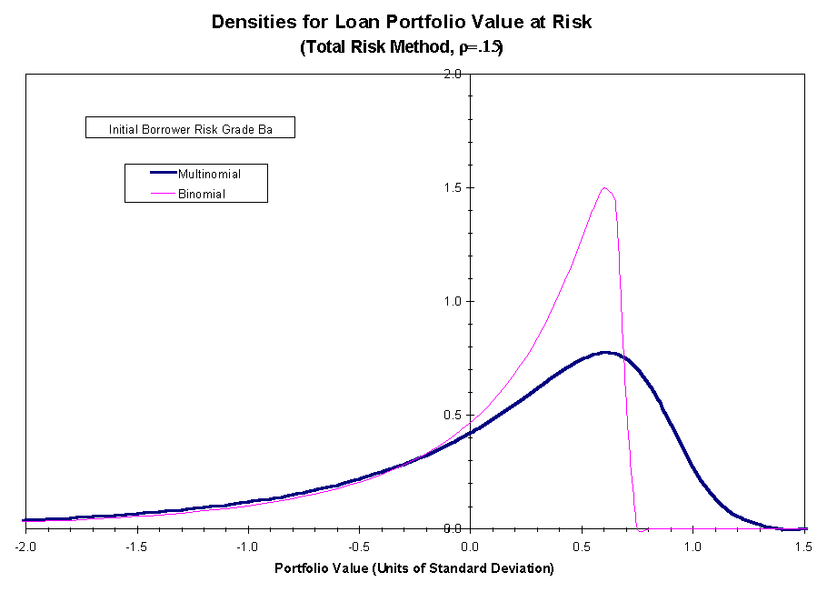
Figure 3
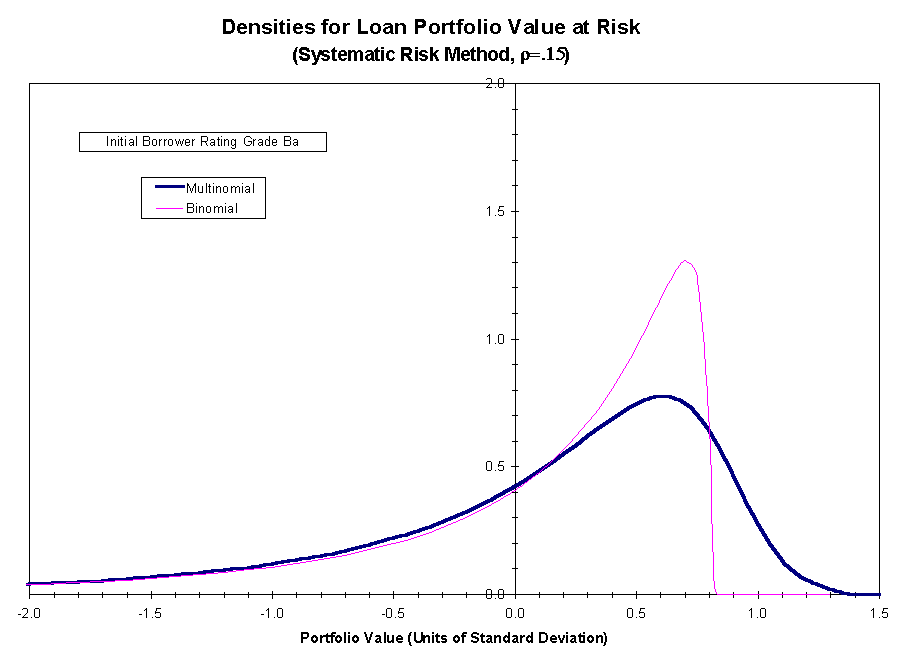
Figure 4
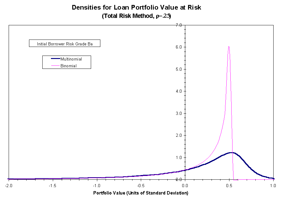
Figure 5
One observes that the par spreads are consistently higher under the systematic risk calibration method. This is consistent with our earlier observation that if the total risk method is used, then the systematic component of loan payoff variance is underestimated. Matching the systematic component of loan variance therefore causes the reference loan to appear more risky. This lowers the loan value to the lender and increases the par credit spreads. The pricing differences are observed to be most signficant in relative terms at the higher rating grades and most significant in absolute terms at the lower rating grades.
Incorporating the systematic risk method into the recursive valuation adds somewhat to the required computation. The key computational steps in imple-menting the scheme we have described are:
(ii) Determine the systematic component
of variance ![]() associated with the possible rating transitions out of each node
associated with the possible rating transitions out of each node ![]() .
.
(iii) Calibrate the reference loan
payoffs ![]() and
and ![]() at
each node to match the mean and systematic variance of the binomial loan
payoff to the mean and systematic variance of the corresponding multinomial
loan payoff.
at
each node to match the mean and systematic variance of the binomial loan
payoff to the mean and systematic variance of the corresponding multinomial
loan payoff.
An alternative less direct method
for estimating ![]() is to take
the Credit-MetricsTM approach and treat rating migration as
driven by asset value movement relative to a default threshold. The procedure
given in [1] for estimating obligor correlations from industry asset correlations
and industry participation weights can then be used.
is to take
the Credit-MetricsTM approach and treat rating migration as
driven by asset value movement relative to a default threshold. The procedure
given in [1] for estimating obligor correlations from industry asset correlations
and industry participation weights can then be used.
Conclusions. It is in the very nature of systematic credit risk that loan transaction credit risk is not "diversified away" even in large loan portfolios. To quantify the effects of systematic credit risk, we have postulated a one-factor model for credit rating migration that separates risk common to all borrowers from risk which is independent from borrower to borrower and therefore diversifiable.
The observed effect of systematic risk at the portfolio level is to cause the (normalized) value-at-risk distribution to take on a distinctly non-Gaussian character. The density mode is skewed significantly to the right, the upper density tail is truncated, and the lower tail is elongated.
We explored the effect on the value-at-risk density of accounting for systematic risk, but distinguishing only between default and non-default in credit rating migration. Our results indicate that the impact on the overall shape of the value-at-risk density is also pronounced. The density which results from this collapse of the non-default states is much more peaked than the actual value-at-risk density and the probability of portfolio loss is underestimated.
Finally, we investigated the impact of systematic risk in the context of applying the methods of arbitrage theory to loan transaction pricing. We analyzed the effect of using total risk as a proxy for systematic risk on the arbitrage pricing of a simple two-period term loan. It was observed that the resulting par credit spreads are lower than those one obtains if proper account is made of the fact that in an arbitrage-free market diversifiable credit risk commands no premium.
References
[2] "Measuring Changes in Corporate Credit Quality," Moody’s Special Report, November 1993
[3] "Debt Rating Migration and the Valuation of Commercial Loans," A. Ginzburg, K. J. Maloney, and R. Willner, Citibank Portfolio Strategies Group Report, December 1994
[4] "Moody’s Ratings Migration and Credit Quality Correlations, 1920-1996," Moody’s Report, 1997
[5] "Martingales and Stochastic
Integrals in the Theory of Continuous Trading," J. M. Harrison and S. R.
Pliska, Stochastic Processes and Their Applications, 11, 1981, pp.
215-260